


A* algorithm tutorial
Download example program for this tutorial (19k)
Download offline version of this tutorial (5k)
About the algorithm
The A* algorithm basicly is a graph search algorithm, but it can also be used as an excellent path-finding algorithm. The main idea is to understand the fields of a map as nodes in a graph. Every node has several neighbouring fields (usually 4 or 8) in straight or diagonal direction. All we need to start with are two nodes: the starting field and the destination field.Open list and closed list
We create two kinds of lists (open and closed) to handle the nodes with. In the open list we put the nodes we are currently working with, and in the closed list the nodes we have already examined. The open list can be defined as any kind of list (i.e. an array) of nodes with the following structure:Position |
(X,Y) coordinate of the node
|
NodeBeforePointer |
Pointer to the node before
|
f |
Distance travelled from the starting node to this node
|
g |
Estimated distance travelling from this node to the destination node
|
h |
Whole distance travelled when arriving at the destination node (sum of f and g)
|
Distance estimation
To calculate g, we have to estimate the distance from the current node to the end node. This estimation has to be optimistic to get the shortest path possible. This means it has to be the shortest way between the two nodes, but we use the optimistic estimation of 0 and set g to 0 for now.Putting the first node into the list
We begin at the starting field, so we put this node in the open list. NodeBeforePointer is a null pointer, f, g and h are 0. The closed list is empty for now because we have not examined any nodes yet.The main loop
The main loop consists of three steps:- searching for the best node in the open list
- putting it in the closed list
- expanding
The second step is to move this node from the open list to the closed list.
In the third step we are adding every possible neighbouring field of the node to the open list.
Adding more nodes
First we have to check if the neighbouring node is already in the open list (that means to check if there is a node with the same position in the list). If it is not in the list we can add the node, but if there is we check if the new node is better (that means if it has a smaller h) and in this case replace the old one.While adding the nodes to the open list we have to set their values. Position is the (X,Y) coordinate. NodeBeforePointer points to the node before, so it points to the node we just came from and which we moved to the closed list. f is the old value of f plus the distance between the old node and the current node (Note: if the path is diagonal, the distance is greater!). g is set to 0 because of the optimistic estimation of 0 and so h is equal to f.
Our goal
We repeat these three steps over and over again until we reach the destination node. This means we have to check if the nodes we added have the same position as the destination node. In this case, we are done. Then we can follow the NodeBeforePointers back to the starting node and get the best path from the starting node to the destination node.Optimizing the algorithm
The path we found is the best, but the algorithm has tested too many nodes. E.g. the path between two points without any obstacles on the map is the line between them, but the algorithm tests many more nodes than those the optimal path goes through.But why does the algorithm test so many nodes? Because of our distance estimation. We have to use an optimistic estimation to find the shortest path, but the optimistic estimation of 0 was way too optimistic.
There is another method of estimation to find the shortest path, the shortest path estimation. This means we set g to the shortest path between the current node and the destination node, which is mathematically speaking the square root of (ΔX˛ + ΔY˛) where ΔX and ΔY are the differences of the nodes coordinates. With this estimation, we get the shortest path between the starting node and the destination node and thus we have to test less nodes than with the too optimistic estimation of 0.
There is a third estimation that tests the smallest number of nodes and thus is the most quickly calculated one. It is the longest path estimation. We simply set g to the longest distance between the starting node and the destination node. This isn't possible when the ground is planar, but if there are different grounds like mud, grass, etc., you can set g to a value as high as if you would go over the worst ground. This estimation is the fastest one, but it will not find the shortest path.
Conclusion
Now that we know a good algorithm for path-finding we can use it in games, simulations or whatever program. To be exact, we actually know two algorithms. The first algorithm uses the shortest path estimation. We can use this algorithm if we want to find the shortest path possible between two points and we don't care about CPU usage. The second algorithm uses the longest path estimation and we can use it to find a path as fast as we can (note that this algorithm can only be used with different grounds - in a planar map the first algorithm is the fastest one).Attention! If there is no way to get from the starting node to the destination node, the two algorithms are both slow. They test every node until there are no more nodes left to test. If the map is very big, this can cause a long calculation time. A way to stop this is to do some precalculations, e.g. marking "islands" of points that can not be connected, as shown here:
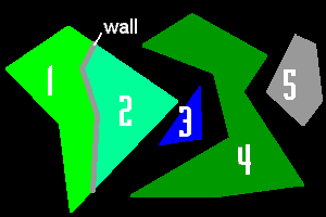
If the destination is on a different "island", it can't be reached